Slurm - Job Script Example 05a TensorFlow With Anaconda Python

An example for using TensorFlow with Anaconda Python <ref name="miniconda_downloads>Anaconda script as a job.

Code

This example is derived from a TensorFlow Core Tutorial on basic image classification.<ref name="tf_tut_imgcls'>TensorFlow Core Tutorials - ML Basics with Keras - Basic classification: Classify images of clothing (Retrieved 2021-05-20) This example uses TensorFlow 2.4 and may not work with other versions of TensorFlow.

We will use the Anaconda Python installed on Picotte to run this example, both on GPUs and on CPUs only.

N.B. your environment will have to be initialized once to setup for use of Anaconda Python. See: Anaconda#URCF-Installed Anaconda

Fashion-MNIST Dataset

This example performs image classification on images of clothing from the Fashion-MNIST dataset.[1] The Fashion-MNIST dataset consists of images with the same format as MNIST data, allowing for a drop-in replacement of the MNIST dataset: they are 28 x 28 grayscale images, concatenated into single files which are then compressed. The Fashion-MNIST dataset has already been downloaded to Picotte: see Sample TensorFlow Datasets#Fashion-MNIST

Python script

The Python script is a file named classify.py:

#!/usr/bin/env python3
import numpy as np
import pandas as pd
import matplotlib.pyplot as plt
import os
import gzip
import time
import random

import tensorflow as tf
from tensorflow import keras

### Source: https://www.tensorflow.org/tutorials/keras/classification

### This was tested using TensorFlow 2.4.1 on CPU-only, and on a single GPU

### TensorFlow automatically uses a GPU if available.
### NOTE To use more than one GPU, that needs to be configured with TensorFlow.
###      While TF may use a single GPU automatically, it will not automatically
###      distribute the computation to multiple GPUs.

def plot_image(i, predictions_array, true_label, img):
    true_label, img = true_label[i], img[i]
    plt.grid(False)
    plt.xticks([])
    plt.yticks([])

    plt.imshow(img, cmap=plt.cm.binary)

    predicted_label = np.argmax(predictions_array)
    if predicted_label == true_label:
        color = 'blue'
    else:
        color = 'red'

    plt.xlabel("{} {:2.0f}% ({})".format(class_names[predicted_label],
                                    100*np.max(predictions_array),
                                    class_names[true_label]),
                                    color=color)


def plot_value_array(i, predictions_array, true_label):
    true_label = true_label[i]
    plt.grid(False)
    plt.xticks(range(10))
    plt.yticks([])
    thisplot = plt.bar(range(10), predictions_array, color="#777777")
    plt.ylim([0, 1])
    predicted_label = np.argmax(predictions_array)

    thisplot[predicted_label].set_color('red')
    thisplot[true_label].set_color('blue')


def load_mnist(path, kind='train'):
    """Load MNIST data from `path`"""
    labels_path = os.path.join(path,
                               '%s-labels-idx1-ubyte.gz'
                               % kind)
    images_path = os.path.join(path,
                               '%s-images-idx3-ubyte.gz'
                               % kind)

    with gzip.open(labels_path, 'rb') as lbpath:
        labels = np.frombuffer(lbpath.read(), dtype=np.uint8,
                               offset=8)

    with gzip.open(images_path, 'rb') as imgpath:
        images = np.frombuffer(imgpath.read(), dtype=np.uint8,
                               offset=16).reshape(len(labels), 784)

    return images, labels


# sanity check
print('')
print(f"TensorFlow version = {tf.__version__}")
print(f"Keras version = {keras.__version__}")
print('')

if tf.test.gpu_device_name():
    print('Connected to GPU(s)', tf.test.gpu_device_name())
else:
    print('Not connected to GPU')
print('')

# load data
train_images, train_labels = load_mnist('/beegfs/Sample_TF_Datasets/Fashion_MNIST', kind='train')
test_images, test_labels = load_mnist('/beegfs/Sample_TF_Datasets/Fashion_MNIST', kind='t10k')

# define class names
class_names = ('T-shirt/top', 'Trouser', 'Pullover', 'Dress', 'Coat', 'Sandal', 'Shirt', 'Sneaker', 'Bag', 'Ankle boot')

print(f'train_images.shape = {train_images.shape}')
print(f'train_labels.shape = {train_labels.shape}')
print(f'test_images.shape = {test_images.shape}')
print(f'test_labels.shape = {test_labels.shape}')
print('')

# normalize images
train_images = train_images / 255.0
test_images = test_images / 255.0

# build model
# NOTE loaded data is already flattened, so we remove the Flatten() layer from the original tutorial
model = tf.keras.Sequential([
    tf.keras.layers.Dense(128, activation='relu'),
    tf.keras.layers.Dense(10)
    ])

# compile model
model.compile(optimizer='adam',
        loss=tf.keras.losses.SparseCategoricalCrossentropy(from_logits=True),
        metrics=['accuracy'])

# train
print('Training starting...')
tic = time.perf_counter()
model.fit(train_images, train_labels, epochs=20)
toc = time.perf_counter()
print('')
print(f'Training completed in {toc - tic:0.4f} seconds')
print('')

# evaluate accuracy
test_loss, test_acc = model.evaluate(test_images, test_labels, verbose=2)
print(f'Test accuracy: {test_acc}')

probability_model = tf.keras.Sequential([model,
    tf.keras.layers.Softmax()])

# verify predictions
predictions = probability_model.predict(test_images)
print(f'predictions[0] = {predictions[0]}')
print(f'highest confidence label = {class_names[np.argmax(predictions[0])]}')
print(f'matching test label = {class_names[test_labels[0]]}')

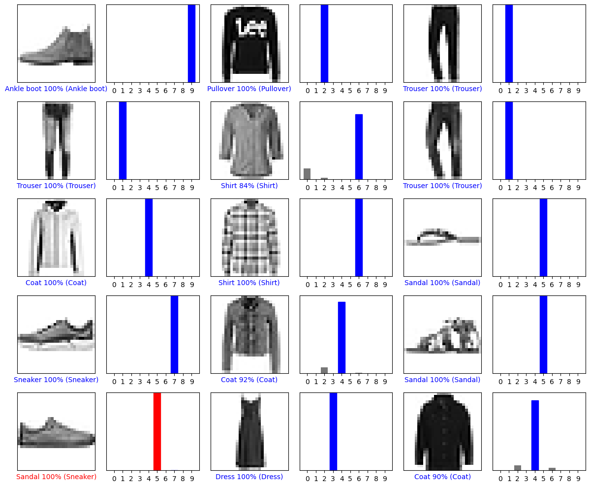
# plot several test images, their predicted labels, and their true labels
test_images_reshaped = np.reshape(test_images, (test_images.shape[0], 28, 28))

num_rows = 5
num_cols = 3
num_images = num_rows * num_cols
fig = plt.figure(figsize=(2*2*num_cols, 2*num_rows))
for i in range(num_images):
    plt.subplot(num_rows, 2*num_cols, 2*i+1)
    plot_image(i, predictions[i], test_labels, test_images_reshaped)
    plt.subplot(num_rows, 2*num_cols, 2*i+2)
    plot_value_array(i, predictions[i], test_labels)
    plt.tight_layout()

plt.savefig('verification.png', bbox_inches='tight')
plt.close(fig)


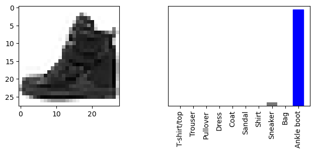
# use the trained model for prediction/inference
print('')
print('Make a prediction on a random image using the model we trained')

# pick an image from test dataset
print(f'There are {test_images.shape[0]} test images')
img_id = random.randint(0, test_images.shape[0])
print(f'Select image no. {img_id}')
img = test_images[img_id]
img_reshaped = np.reshape(img, (28, 28))
print(f'img_reshaped.shape = {img_reshaped.shape}')

# tf.keras models work on a batch of examples. Make a batch of one.
img = (np.expand_dims(img, 0))

predictions_single = probability_model.predict(img)
print(f'Prediction = {class_names[np.argmax(predictions_single[0])]}')

plt.grid(False)
fig = plt.figure()
fig.set_figheight(15)
fig.set_figwidth(8)
plot_value_array(1, predictions_single[0], test_labels)
plt.subplot(num_rows, 2, 1)
plt.imshow(img_reshaped, cmap=plt.cm.binary)
plt.subplot(num_rows, 2, 2)
plot_value_array(0, predictions_single[0], test_labels)
plt.xticks(range(10), class_names, rotation=90)
plt.savefig('prediction.png', bbox_inches='tight')
plt.close(fig)

Job script

The job script is a file named tenEx.sh, in the same directory as classify.py:

#!/bin/bash
#SBATCH -p gpu
#SBATCH --gres=gpu:1
#SBATCH --gres-flags=enforce-binding
#SBATCH --time=1:00:00
#SBATCH --mem-per-gpu=48G

### If running on CPUs only:
### NOTE more cpus-per-task does not mean this will run faster. (You should try it.)
#   #SBATCH -p def
#   #SBATCH --nodes=1
#   #SBATCH --ntasks=1
#   #SBATCH --cpus-per-task=2
#   #SBATCH --time=2:00:00
#   #SBATCH --mem=48G

module load python/anaconda3
. ~/.bashrc

### NOTE
### The above #SBATCH directives need to be modified
### for running on partition "gpu" (using GPUs)
### or partition "def" (using only CPUs)

if [ $SLURM_JOB_PARTITION == "gpu" ]
then
    echo "Running on GPU"
    conda activate tf24-gpu
    nvidia-smi
else
    echo "Running on CPU only"
    conda activate tf24
fi

### check that the correct version of Python is being used

which python3

### NOTE To use more than one GPU, that needs to be configured with TensorFlow.
###      While TF may use a single GPU automatically, it will not automatically
###      distribute the computation to multiple GPUs.

python3 ./classify.py

Job submission

Submit the job script:

[juser@picotte001 ~]$ sbatch tenEx.sh

Output

Generally, GPU will perform many times faster than CPU. (One run completed training in about 33 seconds.)

Output will include a couple of images: verification, and prediction of a randomly selected test image.

Files

Files for these example, except for the logs and outputs, are here:

/ifs/opt/Examples/Example_05a_TensorFlow_with_Anaconda

Note on Performance Tuning for Intel CPUs

Things to note:

1. performance of training this simple model on this small dataset cannot be extrapolated to other models and datasets
2. it is not true that "more cores means faster computation"
3. performance can vary depending on how threads are distributed
4. performance strongly depends on the dataset used

Intel has guidance on setting TensorFlow parameters to distribute work across CPU cores.[2] However, this tuning had little effect on the performance of this simple example.

Performance summary:

No. of GPU devices	No. of CPU cores	Training time (seconds)
0	48	1971.9450
0	24	1839.1679
0	12	1260.2445
0	8	287.8509
0	6	82.1543
0	4	63.4815
0	2	41.2688
0	1	25.5675
1	12*	26.7590
1	2*	29.7021

NOTE * When GPUs are in use, training is performed on the GPUs.

See Also

• Slurm - Job Script Example 05 TensorFlow Singularity
• Slurm - Job Script Example 08 TensorFlow using virtualenv
• Slurm - Job Script Example 08a TensorFlow multi-GPU using virtualenv

References

[1] Zalando Research - Fashion-MNIST GitHub Repository

[2] Intel® Developer Zone - Guide to TensorFlow* Runtime optimizations for CPU